1
Understanding economic mobility across rural America
I compare Census tracts within local labor markets to examine how family, education, and economic characteristics relate to the adult incomes of children raised in low-income families.

2
How tract characteristics relate to economic mobility
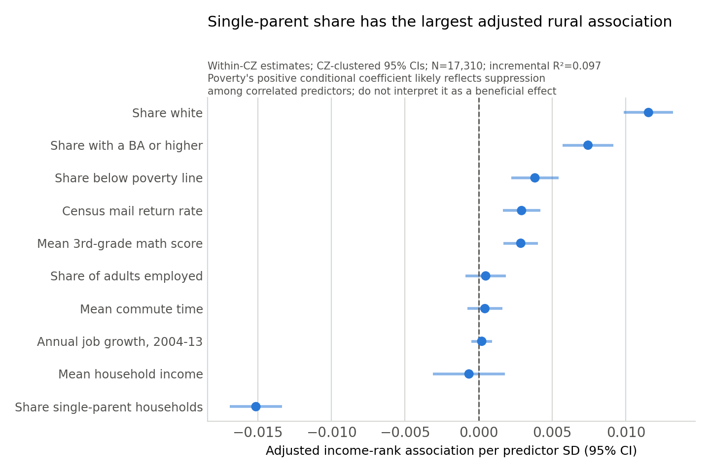
Each point shows the estimated change in the outcome associated with a one-standard-deviation increase in a tract characteristic. The analysis covers 17,310 rural Census tracts, accounts for differences across commuting zones, and shows 95% confidence intervals.
3
Rural vs. Urban
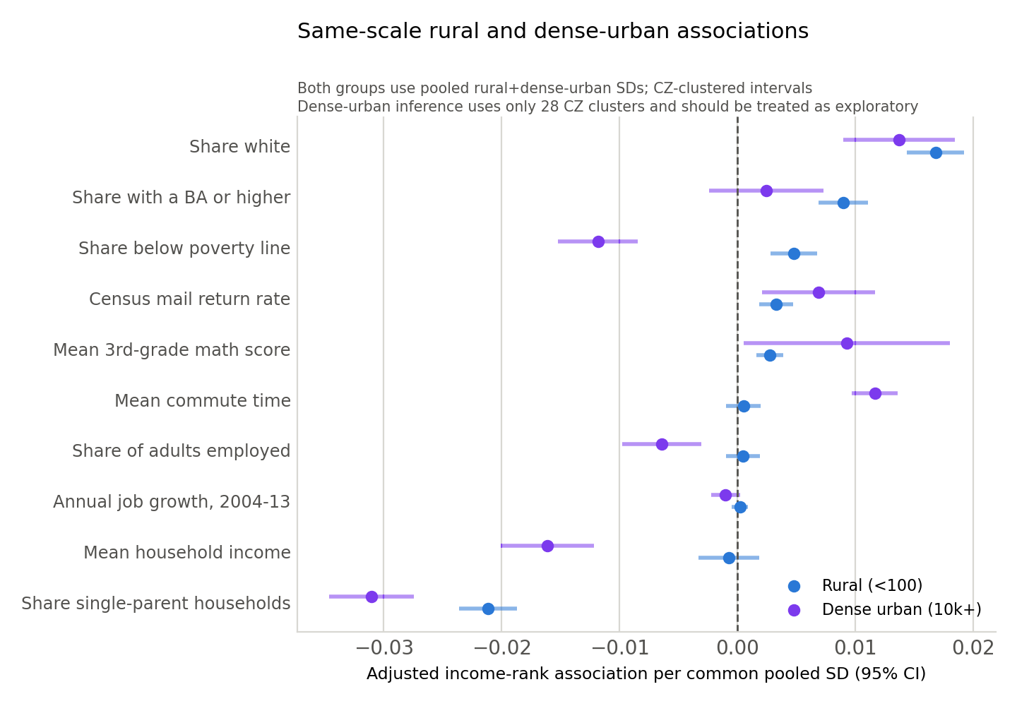
Single-parent share: the negative adjusted association is stronger in dense-urban tracts than in rural tracts.
Share below poverty: the coefficient reverses sign, appearing positive in rural tracts and negative in dense-urban tracts after adjustment.
The data
Opportunity Insights’ Opportunity Atlas, tract tables 4 and 9. The outcome is kfr_pooled_pooled_p25: mean adult household-income rank for children whose parents sat at the 25th percentile, drawn from federal tax records for the 1978–1983 birth cohorts and keyed to the 2010 Census tract where each child grew up.
The raw covariate file holds 74,044 tracts; a validated one-to-one join on (state, county, tract) leaves 71,958 in the analysis sample, spanning 741 commuting zones. I define rural as fewer than 100 people per square mile in 2000 (a transparent project cutoff rather than the Census Bureau’s official classification), which yields 17,978 rural tracts. Models use complete cases and print the resulting row loss.
Full results
| Characteristic (per SD) | Assoc. | 95% CI | p |
|---|---|---|---|
| Share single-parent households | -1.51 | -1.69 to -1.34 | <0.001 |
| Share white | +1.15 | +0.99 to +1.32 | <0.001 |
| Share with a BA or higher | +0.74 | +0.57 to +0.91 | <0.001 |
| Share below poverty line | +0.38 | +0.22 to +0.54 | <0.001 |
| Census mail return rate | +0.29 | +0.16 to +0.42 | <0.001 |
| Mean 3rd-grade math score | +0.29 | +0.17 to +0.40 | <0.001 |
| Share of adults employed | +0.05 | -0.09 to +0.19 | 0.494 |
| Mean commute time | +0.04 | -0.08 to +0.16 | 0.484 |
| Annual job growth, 2004-13 | +0.02 | -0.05 to +0.09 | 0.558 |
| Mean household income | -0.07 | -0.31 to +0.18 | 0.599 |
Percentile points of adult household-income rank per predictor SD. N = 17,310 rural tracts, 727 commuting zones. Commuting-zone indicators alone explain R² = 0.563; the ten characteristics add 0.097 on top of that. This is the honest measure of how much these tract traits explain, and a reminder that most of what predicts mobility here is simply which region you are in.
Rural vs. dense urban
Put rural and dense-urban tracts on one common scale and the rural pattern is not a scaled-down copy of the urban one. Single-parent share leads in both, but income, poverty, and employment behave differently across the two settings. This comparison is exploratory: the dense-urban model contains only 28 commuting-zone clusters, below the point where cluster-robust intervals can be trusted.
What this does not show
Commuting-zone fixed effects handle broad regional composition but not family sorting or unobserved tract differences. The predictors are heavily collinear (income–BA r = 0.78; poverty–income r = 0.64; single-parent–poverty r = 0.62), so any coefficient that flips its bivariate sign is treated as a suppression pattern rather than an independent effect. Several covariates are also measured after the focal cohorts’ childhood years.
The race coefficient is a conditional association on cross-sectional tract data, consistent with the documented national race gaps in mobility, but not interpretable as a place effect under this design.
Reproduce it
Three notebooks run in numeric order from code/. Each defines its functions at the top and imports shared paths from utils.py, so nothing is hardcoded to one machine. Raw data are not committed; 00_pull.ipynb re-downloads them, so a fresh clone reproduces every figure and table on this page.
- 00_pull.ipynb
Downloads Opportunity Atlas tables 4 and 9; prints row counts, duplicate-id checks, and missing-cell counts.
- 01_merge.ipynb
Validates a one-to-one join on (state, county, tract), prints row-loss diagnostics, builds density categories, audits missing cells.
- 02_analyze.ipynb
Fits standardized OLS with commuting-zone fixed effects and CZ-clustered SEs, runs the 200-child screen and the dense-urban comparison, writes every figure and table.